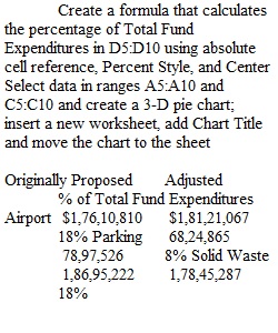
Q PC Users PC users with Office 2016 or 2013 or 365 follow directions in Excel Chapter 3 Analyzing Data with Pie Charts, Line Charts, and What-If Analysis Tools to create Project 3A. e03A_Enterprise_Fund.xlsx Download e03A_Enterprise_Fund.xlsx Project: 3A_Enterprise_Fund Task Points Create a formula that calculates the percentage of Total Fund Expenditures in D5:D10 using absolute cell reference, Percent Style, and Center 2 Select data in ranges A5:A10 and C5:C10 and create a 3-D pie chart; insert a new worksheet, add Chart Title and move the chart to the sheet 2 Retitle the chart Enterprise Fund Expenditures, apply WordArt style Fill Gold, Accent 4, Soft Bevel to title, change font size to 32 1 Format data labels to display categories and percentages; Center labels, apply Bold Italic font, resize to 11 pt 2 Format the 3-D chart with Circle bevel, Top and Bottom Bevel width and height set to 512; material, Standard Plastic; add a shadow to the chart 2 Rotate the pie chart and explode a slice 10%, change slice color to Waterfront, Gradient Fill, Bottom Spotlight, Accent 6 2 Format the chart area with background gradient fill, Bottom Spotlight, Accent 1, Solid line border, border color Blue-Gray, Text 2, width 5pt 2 Edit worksheet data to update the chart, increasing Airport to 18% on the pie chart 2 Use Goal Seek and perform What-If Analysis for 9% goal on Expenditures Worksheet; Enter Goal row title text, merge and center across range A13:D13, Heading 3 Cell Style; enter goal amount in B14 2 Add shading to Goal Amount on worksheet by changing themed cell style of range A14:C14 to 20%, Accent 1; change B14 to Number Format, Currency with no decimal places 1 Center the page horizontally 1 Insert footer with file name, add document properties with name and keywords 1 Total Points 20 Copyright © 2014 Pearson Education, Inc. Publishing as Prentice Hall Mac Users Mac users with Office 2016 or 2011 or 365 follow directions in Excel Chapter 3 Analyzing Data with Pie Charts, Line Charts, and What-If Analysis Tools to create Project 3A. e03A_Fund_Expenses.xlsx Download e03A_Fund_Expenses.xlsx Project: 3A_Fund_Expenses Task Points Calculate percentage by which the values make up the total in D5:D10, apply percent style and center 3 Select data and create 3-D pie chart on new sheet 2 Apply category names and percentages to labels and format, add chart title and format, remove legend 2 Format pie chart with 3-D bevel options and shadow effect 2 Rotate the pie chart and explode and color Administrative pie slice 2 Format the chart area with bevel shape effect and background gradient 1 Insert text box with text Goal: Reduce Administrative to 8% 1 Edit worksheet data to update the chart 2 Insert WordArt in worksheet, font size 28 1 Type title and heading, copy C9:D9 and paste to B18:C18. Use Goal Seek to estimate reduced Administrative expense, apply styles and formatting per instructions 2 Rename Sheet1 and remove unused worksheets 1 Insert footer with file name, add document properties with name and keywords, page layout in Portrait and centered horizontally 1 Total Points 20 Copyright © 2013 Pearson Education, Inc. Publishing as Prentice Hall PreviousNext
View Related Questions